Basic Statistical Terminology

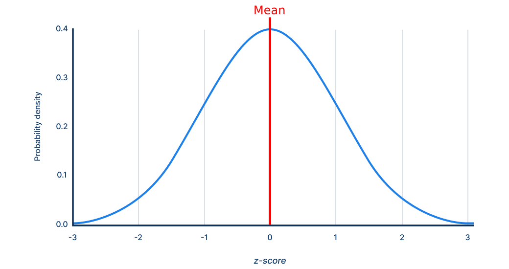
Mean

Definition: The arithmetic average of a set of scores. It is obtained by adding all observations ($\sum x$) and dividing by the total number of observations ($N$):

$$\mu = \frac{\sum_{i=1}^{N} x_i}{N}$$

Where

• $x_i$ = the i-th individual score in the data set
• $N$ = the total number of scores (sample size)

In psychometric norm tables, the mean anchors the scale- for example, most modern IQ tests set the population mean at 100. On a normal or Gaussian distribution, the mean represents the 50th percentile.

---

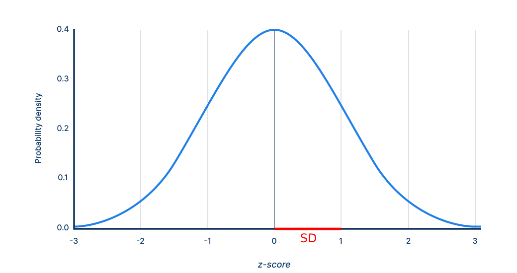
Standard Deviation (SD)

Definition: A measure of score dispersion that indicates, on average, how far each score lies from the mean. It is the square root of the mean of squared deviations:

$$\sigma = \sqrt{\frac{\sum_{i=1}^{N} (x_i - \mu)^2}{N}}$$

Where

• $x_i$ = the i-th individual score in the data set
• $\mu$ = the mean (arithmetic average) of all scores
• $N$ = the total number of scores (sample size)

Larger SDs signify greater variability. On many IQ scales, 1 SD = 15 points, so a score of 115 is one SD above the mean of 100. On a normal or Gaussian distribution, an SD is represented by horizontal bands of equal width as below.

---

Correlation $r$

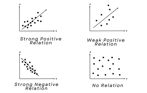
Definition: The correlation coefficient quantifies the strength and direction of a linear relationship between two continuous variables. Values range from -1 (perfect inverse) through 0 (no linear association) to +1 (perfect direct association). Correlation is foundational to concepts such as reliability, validity, factor analysis, and linear regression, yet a high $r$ does not imply causation.

For a sample of size $N$:

$$r \;=\; \frac{\displaystyle\sum_{i=1}^{N}(x_i - \bar{x})(y_i - \bar{y})} {\sqrt{\displaystyle\sum_{i=1}^{N}(x_i - \bar{x})^{2}} \;\sqrt{\displaystyle\sum_{i=1}^{N}(y_i - \bar{y})^{2}}}$$

Where

• $x_i,\;y_i$ = paired scores for observation $i$
• $\bar{x},\;\bar{y}$ = sample means

Direction: Positive $r$ → as $X$ increases, $Y$ tends to increase; negative $r$ → $Y$ tends to decrease.

Proportion of shared variance: (r^2) (the coefficient of determination) indicates the percentage of variance in one variable linearly explained by the other.

Example: $r=0.60 \Rightarrow r^{2}=0.36$, 36% of the variance is shared.

---

Variance $r^2$

Definition: is the proportion of total score variance that is accounted for by a predictor (in simple correlation) or by the full set of predictors in a regression or factor model. It can be interpreted as "the percentage of variance between test scores between different testees that is explained by the latent factor".

You can get this value by squaring the correlation.

Example: $r=0.60 \Rightarrow r^{2}=0.36$

$r^{2} = 0.36$ means the model (or single predictor) explains 36% of the variance in the outcome; the remaining 64 % is unexplained (error or other factors).

---

Raw Score

Definition: The examinee's observed or obtained score, the simple count of points earned or items answered correctly before any statistical adjustment. Raw scores are sample-dependent and therefore cannot be compared meaningfully across age groups, different test editions, or separate forms until they are converted to a common metric (e.g., a standard score).

---

Standard Score

Definition: A transformed score that expresses an individual's performance in units of the population's standard deviation (SD) around a chosen mean (often 100). For most IQ scales a score of 100 represents the mean of the norm (usually white Americans/Brits depending on the test) and every 15-point increment above or below reflects one SD. Standard scores make it possible to:

1. compare results from different subtests or batteries,
2. track growth over time, and
3. communicate results without revealing raw items.

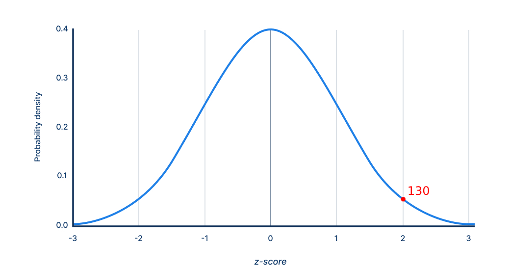
A standard score of 130 is 2 standard deviations above the mean.

---

Z-Score

Definition: A linear standard score computed as

$$z = \frac{X-M}{SD}$$

where $X$ is the raw score, $M$ is the reference-group mean, and $SD$ is its standard deviation. Z-scores have a mean of 0 and $SD = 1$, allowing direct lookup of cumulative probabilities under the normal curve. They form the mathematical basis for almost every other standard-score family (T, scaled, IQ, stanine).

A simple way to view it is that a Z score is the number of standard deviations the score is above or below the mean, e.g. a z-score of 0.67 would be 0.67 standard deviations above the mean while a z-score of -1.5 would be 1.5 standard deviations below the mean.

---

T-Score

Definition: A derivative of the z-score with a mean of 50 and $SD = 10$:

$$T = 10z + 50$$

T-scores avoid negative values and decimals, making them popular in personality, clinical, and neuropsychological scales. A $T=60$ is one SD above the mean; $T=70$ is two SDs above, and so on.

---

Scaled Score (SS)

Definition: A derivative of the z-score with a mean of 10 and SD of 3:

$$SS = 3z + 10$$

Many cognitive batteries (such as the WAIS and WISC) report scaled scores for individual subtests because those subtests contain relatively few items and therefore have lower reliability; using a coarse 1 - 19 scale (M = 10, SD = 3) prevents test users from over-interpreting differences that are mostly measurement error. $SS$ of 11 is 105 IQ; $SS$ of 12 is 110 IQ, and so on.

---

Composite Scores

Definition: The summation of scaled scores used to form a composite score, e.g., an overall Full Scale IQ. This is calculated by summing the SS from multiple subtests, known as SSS (Sum of Scaled Scores). The SS is then referred to a look-up table to find its corresponding composite IQ scores. These composite scores can represent specific cognitive abilities like verbal and fluid reasoning IQ, or Full-Scale IQ.

As for norming, the composite scores are compared to a representative sample of the population. In norming, some basic steps are followed, such as calculating the mean and SD of the composite scores in the norm group and establishing the percentiles. These scores allow for the interpretation of an individual's performance relative to the general population.

---

Percentile Rank

Definition: The percentage of the normative sample that scores below a given raw or transformed score. For example, the 84th percentile means the examinee outperformed 84% of the reference group. Percentile ranks are ordinal, not interval, so differences between adjacent percentiles vary in raw-score magnitude (e.g., a jump from the 1st to the 2nd percentile is far smaller in raw points than a jump from the 50th to the 51st). A z-score of 1 is the 84%ile, a z-score of 2 is the 98%ile, and so on.

---

Stanine

Definition: Short for "standard nine," the stanine scale divides the normal distribution into nine ordinal bands (1-9) with a mean of 5 and an SD of ≈ 2. Each band except the extremes (1 and 9) captures roughly half an SD.

Stanines furnish a quick verbal descriptor (e.g., very low (1-2), low (3), below average (4), average (5), etc.) and are useful in school settings.

---

Norm Group

Definition: The carefully selected, demographically balanced population whose data are used to derive norms (means, SDs, percentile cuts). A valid norm group mirrors the test taker on key variables which can influence test accuracy such as age, grade, language, nationality, etc. A mismatch can lead to non-equivalent interpretations.

---

Reliability

Definition: A ratio of true-score variance to observed-score variance,

$$r = \frac{\sigma_T^{2}}{\sigma_X^{2}}$$

that quantifies score consistency on a 0 - 1 scale. Coefficients ≥ .90 are desirable for high-stakes individual decisions (eligibility, diagnosis); coefficients around .80 may suffice for group research. Common flavors include internal consistency (α), test-retest, and split-half.

---

Cronbach's α

Definition: An internal-consistency index reflecting the average correlation among all possible split-halves of a multi-item scale, corrected for length. Values rise as items measure the same underlying construct and as the number of items grows. However, α assumes unidimensionality; a high α does not by itself prove validity.

$$\alpha \;=\; \frac{K}{K - 1}\! \left( 1 - \frac{\displaystyle\sum_{i=1}^{K} \sigma_i^{2}} {\sigma_{T}^{2}} \right)$$

Where

• $K$ = number of items (test questions or scale indicators)
• $\sigma_i^{2}$ = variance of item $i$
• $\sigma_{T}^{2}$ = variance of the total (sum) score across the $K$ items

---

Split-Half Reliability

Definition: Correlation between two halves of a test-often odd vs. even items-expanded to full length via the Spearman-Brown formula. It is faster to compute than α but sensitive to how the test is split.

$$r_{\text{SB}} \;=\; \frac{k\,r}{1 + (k - 1)\,r}$$

Where

• $r_{\text{SB}}$ = predicted reliability of the full-length test after applying the Spearman-Brown correction
• $r$ = Pearson correlation between the two halves of the test
• $k$ = length‐adjustment factor
  • For split-half reliability, $k = 2$ (because two halves)
  • For other length changes, $k$ equals the ratio of the new test length to the original length

---

Test-Retest Reliability

Definition: Correlation of scores obtained from the same individuals on two administrations separated by a defined interval (days, weeks, months). High values indicate temporal stability; lower values may reflect learning, fatigue, or construct change.

---

Standard Error of Measurement (SEM)

Definition: The standard deviation of an examinee's hypothetical score distribution across infinite parallel forms:

$$\text{SEM} \;=\; \sigma \,\sqrt{1 - r_{xx}}$$

Where

• $\sigma$ = standard deviation of scores in the normative population
• $r_{xx}$ = reliability coefficient of the test

A single IQ point estimate is best interpreted as a range. The observed score $±1×SEM$, returns ~68% confidence intervals, while observed score $±2×SEM$ returns ~95% confidence intervals.

---

Validity

Definition: The quality of evidence supporting the interpretation, use, and consequences of test scores. Modern validity is unitary but draws on multiple sources:

• Construct validity - how well does the test measure its construct? Usually measured through measuring how much of the variance is attributable to the first factor through principle components analysis or factor analysis.
• Convergent validity - is the test measuring the same latent factor it intends to measure? Usually measured through correlations to scores on other proven measures of the intended latent factor.
• Discriminant validity - is the test only measuring the intended factor and not an unrelated one? Measured by verifying the test has low correlations with unrelated traits (e.g. Big-Five).
• Criterion validity - what is the extent to which test scores correspond to an external criterion?
  • Predictive validity: how well scores forecast future outcomes that are meaningful and consistent (e.g., later job performance, GPA, or clinical diagnosis).
  • Concurrent validity: how well scores correlate with a criterion that is measured at the same time (e.g., a well-established test administered on the same day).

Without sufficient validity evidence, high reliability merely indicates consistent error.

---

Construct

Definition: An abstract psychological attribute (e.g., fluid reasoning, working memory) that cannot be observed directly but is inferred from behavior or responses. Clear construct definitions drive item writing, scoring, and theoretical interpretation.

---

Factor / Latent Variable

Definition: An unobserved dimension that explains the shared variance among observed indicators (items or subtests).

In context: CHC theory
Modern IQ tests (e.g., WISC-V, SB-5, Woodcock-Johnson IV) adopt the CHC theory:

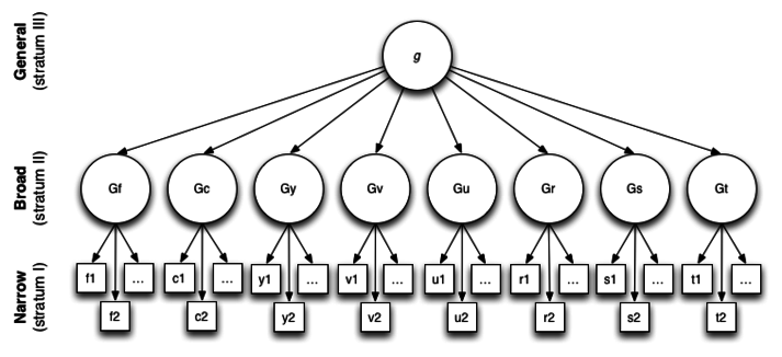
1. Stratum III: a single general factor (g) accounting for the largest share of common variance.
2. Stratum II: broad abilities such as Gf (fluid reasoning), Gc (crystallized knowledge), Gv (visual-spatial), Ga (auditory processing), Gs (processing speed), Gwm (working memory), and Glr (long-term retrieval).
3. Stratum I: dozens of narrow factors (e.g., spatial relations, phonetic coding) represented by individual subtests.

Each latent factor is unobserved, we infer its presence because scores on relevant subtests cluster together more tightly than chance would predict.

---

Factor Analysis (EFA / CFA)

Definition: Statistical techniques for modeling latent structure:

• Exploratory Factor Analysis (EFA) uncovers the number and pattern of factors without strict prior hypotheses.
• Confirmatory Factor Analysis (CFA) tests whether data fit a pre-specified model (e.g., a hierarchical CHC structure). Fit indices (CFI, RMSEA, SRMR) gauge if the data fits the model adequately.

Here's an example of a second-order hierarchical factor model, for the WAIS-IV.

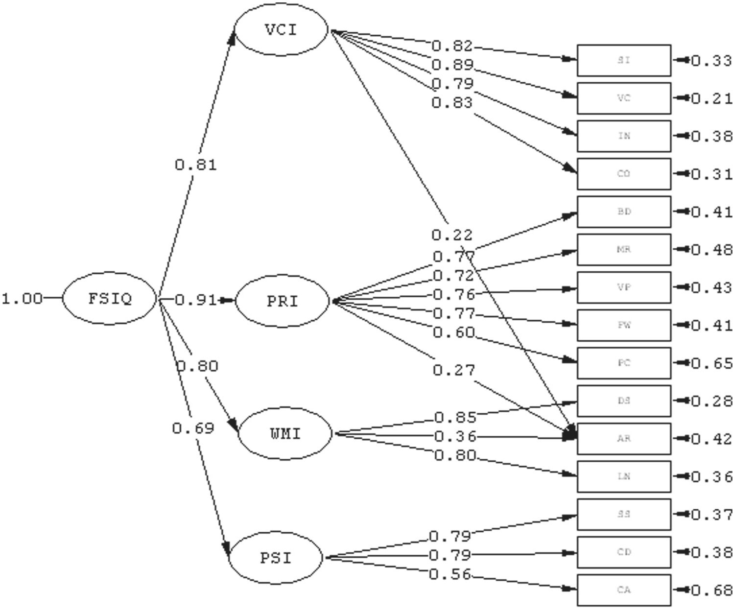
At the top of the hierarchy, the general intelligence factor FSIQ (interpretable as g) loads on the four broad ability indices (VCI, PRI, WMI, and PSI) with standardized coefficients ranging from 0.69 to 0.91. These large coefficients indicate that most of the reliable variance in each broad index is accounted for by the higher-order g factor.

The arrows pointing into each rectangular subtest box represent error terms, which are unique variance and measurement error that remain unexplained by the common factors. Even strongly loading subtests retain item-specific variance.

---

Item Response Theory (IRT)

Definition: A family of probabilistic models that link the likelihood of a correct response ($P$) to an examinee's ability ($\theta$) and item parameters:

• $a$ (discrimination) - slope of the curve (What percentage of each ability level gets this problem correct?)
• $b$ (difficulty) - location along $\theta$ (What is the average ability level who gets this problem correct?)
• $c$ (guessing) - lower asymptote in 3-PL models

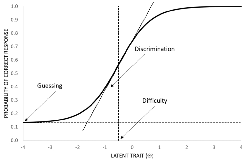
IRT yields sample-independent ability estimates, item information functions, and enables computerized adaptive testing.

---

Classical Test Theory (CTT)

Definition: The traditional model in which the observed score satisfies

$$X = T + E$$

with $T$ the true score and $E$ random error. While conceptually intuitive and computationally simple, CTT statistics (e.g., α, SEM) are sample-dependent and assume all items contribute equally.